
What are explorers looking for in S.A.? Part 2

Spatially assessing the distribution of exploration topics using python.
In the previous article, I demonstrated an application of NLP topic modelling using Latent Dirichlet Allocation and the Gensim library to identify themes in South Australian exploration report summaries. That ML model identified eight coherent topics in the report data set that closely aligns with my domain knowledge of the types of exploration undertaken in the State, and demonstrates some of the potential of undertaking this type of analysis on unstructured geological reports.
As a geologist by trade, I often tend to think about things spatially. Where (and when) do things occur and how does that relate to other observables. To that end I decided to try and represent the spatial distribution of those eight identified topics and see if they align with what I know about the geology and exploration potential of SA. In this second part of “What are explorers looking for in SA”, I will go through one process of creating a spatially enabled data set of exploration reports using the geopandas library and then plotting them with the geoplot and contextily libraries.
Creating the tenement data set
In the previous article, we used the index data set of the South Australian exploration reports provided by the South Australian Department for Energy and Mining, freely available from the SARIG web portal. This csv file contains a number of metadata columns about each exploration report including the envelope number (the document ID), the tenement number associated with the report, a broad subject and a short summary or abstract of the report, along with a number of other metadata columns. The important data column for the previous topic modelling article was the abstract column, consisting of a short text summary of the envelope created by a GSSA geologist. We then added to this data set by processing the abstracts for the LDA modelling and finally appending the results of the model. For this article, we will focus on the tenement number to allow us to put spatial constraints on each exploration report.
First, let’s import the python libraries we’ll need and then open up and have a look at the final data set produced previously:
import pandas as pd
import numpy as np
import matplotlib.pyplot as plt
import seaborn as sns
import geopandas as gpd
import contextily as ctx
import geoplot as gplt
import os
sns.set_style("darkgrid")
pd.set_option('max_columns', 30)
pd.set_option('display.max_colwidth', 200)
final_LDA_df = pd.read_csv(r'D:\Python ML\Envelope-key-words\Data\Processed\Envelope_modelled_topics_20201127.csv').drop(['Unnamed: 0'], axis=1)

final_LDA_df.info()
<class 'pandas.core.frame.DataFrame'>
RangeIndex: 5894 entries, 0 to 5893
Data columns (total 16 columns):
 #   Column               Non-Null Count  Dtype
---  ------               --------------  -----
 0   ID                   5894 non-null   object
 1   Category             5894 non-null   object
 2   Title                5894 non-null   object
 3   Publication Date     5630 non-null   object
 4   Format               5886 non-null   object
 5   Broad Subject        5892 non-null   object
 6   Notes                2753 non-null   object
 7   Tenement             5465 non-null   object
 8   normalised_Abstract  5894 non-null   object
 9   Abstract_toks        5894 non-null   object
 10  Abstract_len         5894 non-null   int64
 11  Dominant_Topic       5894 non-null   float64
 12  Percent_Contrib      5894 non-null   float64
 13  Topic_keywords       5894 non-null   object
 14  Topic_Name           5894 non-null   object
 15  Relevent_words       5894 non-null   object
dtypes: float64(2), int64(1), object(13)
memory usage: 736.9+ KB
final_LDA_df.sample(1)
| ID | Category | Title | Publication Date | Format | Broad Subject | Notes | Tenement | normalised_Abstract | Abstract_toks | Abstract_len | Dominant_Topic | Percent_Contrib | Topic_keywords | Topic_Name | Relevent_words | |
|---|---|---|---|---|---|---|---|---|---|---|---|---|---|---|---|---|
| 162 | ENV00407 | Company mineral exploration licence reports | Moonta-Wallaroo area. Progress reports to licence expiry/renewal, for the period 1/9/1963 to 31/8/1965. | 24-Sep-64 | Digital Hard Copy Hard Copy | Mineral exploration - SA; Drilling; Geophysics; Geochemistry | Continuation of tenure over same area formerly held as SML 42. Please refer to Env 6999 to see SML 59 six-monthly reports ... | SML00059 | report discuss ongoing geophysical geochemical diamond drilling investigation regional magnetic feature around northern end yorke peninsula targette hide supergene copper gold mineralisation moont... | ['report', 'discuss', 'ongoing', 'geophysical', 'geochemical', 'diamond', 'drilling', 'investigation', 'regional', 'magnetic', 'feature', 'around', 'northern', 'end', 'yorke', 'peninsula', 'target... | 61 | 2.0 | 0.4413 | gold' sample' mineralisation' hole' copper' area' prospect' drilling' sampling' rock | Gold, copper, base metal exploration | ['gold', 'soil', 'sample', 'rock_chip', 'copper', 'value', 'sampling', 'au', 'base_metal', 'mineralisation', 'anomalous', 'geochemical', 'return', 'assay', 'vein', 'prospect', 'ppm', 'zone', 'bedr... |
From the above we can see that there are 16 columns of data in this data set. For the present exercise, we don’t need all this information. So lets make a new DataFrame which only contains the data we need for the spatial modelling, namely the ID, tenement number and the modelling results:
tenements_df = final_LDA_df[['ID', 'Tenement','Dominant_Topic','Topic_Name']]

tenements_df.info()
<class 'pandas.core.frame.DataFrame'>
RangeIndex: 5894 entries, 0 to 5893
Data columns (total 4 columns):
 #   Column          Non-Null Count  Dtype
---  ------          --------------  -----
 0   ID              5894 non-null   object
 1   Tenement        5465 non-null   object
 2   Dominant_Topic  5894 non-null   float64
 3   Topic_Name      5894 non-null   object
dtypes: float64(1), object(3)
memory usage: 184.3+ KB
tenements_df.sample(3)
| ID | Tenement | Dominant_Topic | Topic_Name | |
|---|---|---|---|---|
| 1025 | ENV02325 | EL00085;EL00087;EL00121 | 1.0 | IOCG exploration |
| 3413 | ENV08917 | EL01858 | 2.0 | Gold, copper, base metal exploration |
| 2652 | ENV06685 | NaN | 4.0 | Mine operations and development |
There are a number of things to note about this new DataFrame. Not every envelope that has an abstract has an associated tenement number, in fact there are 5894 rows in this data set but only 5465 have tenement numbers. Those reports without tenement numbers would relate to departmental or university publications that aren’t explicitly linked to a physical tenement.
The other thing to note is some of the reports have multiple tenement numbers associated with them. This may be because of a number of things, such as renewals, the tenement changing hands or the tenement type may change from say an exploration lease to a mining lease etc. Another reason may be that the report refers to a number of separate tenements that are held by the same company and are reported against as a group under an amalgamated expenditure agreement.
To deal with this I decided to try two different options and see how many of these tenement numbers I could match up to physical spatial boundaries. One was to use the entire list of tenement numbers and the other was to only use the most recent (highest number) to represent the location of the report. To get this we can first create a list of individual tenement numbers by using the split method on the ‘;’ deliminator and then create a new ‘most_recent_tenement’ column containing only the last one:
tenements_df['Tenement'] = tenements_df['Tenement'].str.split(';')
tenements_df['most_recent_tenement'] = tenements_df.Tenement.str[-1]
tenements_df.tail(3)
| ID | Tenement | Dominant_Topic | Topic_Name | most_recent_tenement | |
|---|---|---|---|---|---|
| 5887 | ENV13185 | [EL02593, EL03221, EL04388, EL05542] | 6.0 | Heavy minerals, ?extractives and environmental | EL05542 |
| 5889 | ENV13201 | [EL02692, EL03346, EL04597, EL05773] | 2.0 | Gold, copper, base metal exploration | EL05773 |
| 5893 | ENV9267 | [OEL00020, OEL00021, PEL00005, PEL00006, PPL00014] | 4.0 | Mine operations and development | PPL00014 |
We can then make an assessment of just how many different tenement types and individual tenement numbers there are in our data set:
all_tenements_exploded = tenements_df.explode('Tenement')
all_tenements_exploded['tenement_type'] = all_tenements_exploded['Tenement'].str.extract(r'(^\D{1,3})')
# and just for the most recent temenments
tenements_df['tenement_type'] = tenements_df['most_recent_tenement'].str.extract(r'(^\D{1,3})')
all_tenements_exploded['tenement_type'].value_counts()
EL     6933
SML     837
PEL     746
MC      327
ML      310
GEL     274
OEL     227
PPL     177
EPP     146
ATP      20
PE       17
PEP      16
PM       14
RL       10
MSL      10
THR       7
MR        5
MPL       5
ELA       5
PRL       5
EML       4
AAL       3
T         2
SA        1
FR        1
OP        1
SIP       1
Name: tenement_type, dtype: int64
We can then create a list of tenement numbers to see how many we have, and to use later in selecting our spatial boundaries:
most_recent_tenem_list = tenements_df['most_recent_tenement'].dropna().to_list()
all_tenements_list = all_tenements_exploded['Tenement'].dropna().to_list()

print(len(most_recent_tenem_list))
print(len(all_tenemenents_list))
5465
10109
So there are 5465 most recent tenements (as expected this is the same number of exploration reports that have an associated tenement number), and over 10,000 tenement numbers in total. We can see from the value counts above that this is dominated by the EL (Exploration Licence) type for mineral exploration with nearly 7000 tenements, followed by SML (Special Mining Lease), PEL (Petroleum Exploration Licence), MC (Mineral Claim), ML (Mining Licence), GEL (Geothermal Exploration Licence), OEL (Oil Exploration Licence), PPL (Petroleum Production Licence) and EPP (Exploration Permit for Petroleum) each with between 1000 and 100 tenements.
Now we have the tenement numbers associated with our exploration report topics, we need to get the spatial data sets so we can make some maps.
Downloading the tenement spatial data
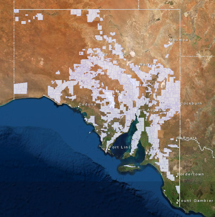
I’ve used the word tenement a lot so far in this article, but what exactly is a tenement. When an exploration company want’s to explore for resources, they are required by law to ‘peg’ a mineral claim. Back before gps and digital systems, this meant exactly that, they would physically peg out the boundaries of their mineral claim. Now days this is all done online through application via the SARIG web portal where applicants can digitally draw the area onto a map, with the exact coordinates being captured. The below image is a snapshot of the current mineral exploration licence tenements from SARIG as at January 2021.
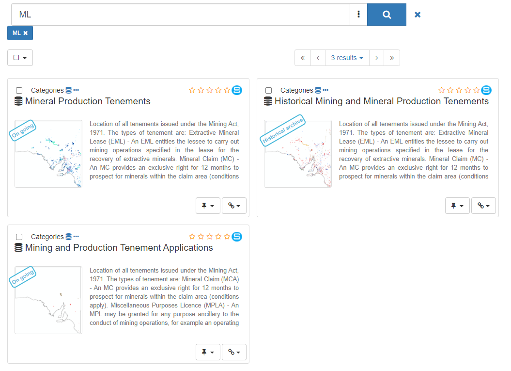
The spatial boundaries of each tenement (active and historic) are provided as polygons in a variety of formats including as an ESRI Geodatabase or SHP file, a MapInfo TAB file and a Google Earth KMZ file. The easiest way to download the tenement data is via the SARIG catalog.
Here I searched for each tenement type, focussing on the ones that had over 100 records. It’s important to note here that there are generally two or three files for each tenement type, one with the current records, one which contains the aggregated historic records and sometimes one with the current applications for new tenements. It’s also important to note that some of the files include more that a single tenement type, for example the ‘Historical Mining and Mineral Production Tenements’ file contains data for EML’s, MC’s, ML’s, MPL’s, PM’s, RL’s and SML’s.
geopandas library: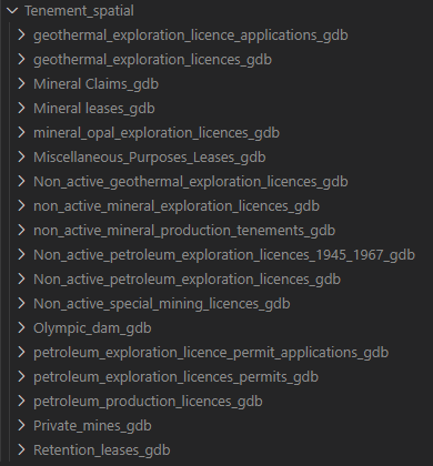
Creating a spatial dataframe
The next step in the process is to extract the required spatial data from the ‘gdb’ files so we can append it to our exploration report dataframe. This is where the geopandas library comes in. geopandas is an open source project built on pandas and shapely to make working with geospatial data in python easy. Because it’s built on pandas, the api is very similar and working between the two is really easy.
First we need to create a geopandas GeoDataFrame for each of our ‘gdb’ files. To do this we can iterate over all the ‘gdb’ files in the folder and append each into a python dictionary, using the ‘gdb’ folder name as the key:
tenm_path = (r'D:\Python ML\Envelope-key-words\Data\Tenement_spatial')

tenm_dict = {}
for root, dirs, files in os.walk(tenm_path):
    for dir in dirs:
        if dir.endswith(".gdb"):
            key = dir
            data = gpd.read_file(os.path.join(root,dir))
            tenm_dict[key] = data

tenm_dict.keys()
dict_keys(['geothermal_exploration_licences.gdb', 'geothermal_exploration_licence_applications.gdb', 'Mineral Claims.gdb', 'Mineral leases.gdb', 'mineral_opal_exploration_licences.gdb', 'Miscellaneous_Purposes_Leases.gdb', 'Non_active_geothermal_exploration_licences.gdb', 'non_active_mineral_exploration_licences.gdb', 'non_active_mineral_production_tenements.gdb', 'Non_active_petroleum_exploration_licences_1945_1967.gdb', 'Non_active_petroleum_exploration_licences.gdb', 'Non_active_special_mining_licences.gdb', 'Olympic_dam.gdb', 'petroleum_exploration_licences_permits.gdb', 'petroleum_exploration_licence_permit_applications.gdb', 'petroleum_production_licences.gdb', 'Private_mines.gdb', 'Retention_leases.gdb'])
Now we have a dictionary of GeoDataFrames we need to take a look at them and see what data we have and how it is presented. The geometry column, with a data type of ‘geometry’ is where all the geopandas magic lies. This column holds the spatial attributes, in this case polygons, for our tenement boundaries. For us to be able to join the spatial data onto our exploration topic DataFrame we will need to use the tenement numbers as the join key.
tenm_dict['Retention_leases.gdb'].info()
<class 'geopandas.geodataframe.GeoDataFrame'>
RangeIndex: 28 entries, 0 to 27
Data columns (total 26 columns):
 #   Column                       Non-Null Count  Dtype
---  ------                       --------------  -----
 0   OBJECTID                     28 non-null     int64
 1   TENEMENT_TYPE                28 non-null     object
 2   Reports_and_related_records  28 non-null     int64
 3   TENEMENT_LABEL               28 non-null     object
 4   TENEMENT_STATUS              28 non-null     object
 5   TENEMENT_HOLDERS             28 non-null     object
 6   TENEMENT_OPERATORS           28 non-null     object
 7   LEGAL_AREA                   28 non-null     float64
 8   AREA_UNIT                    28 non-null     object
 9   LOCATION                     18 non-null     object
 10  REGISTRATION_GRANT_DATE      28 non-null     object
 11  SURRENDER_DATE               0 non-null      object
 12  EXPIRY_DATE                  28 non-null     object
 13  RENEWAL_RECEIVED_DATE        7 non-null      object
 14  TRANSFER_RECEIVED_DATE       2 non-null      object
 15  SURRENDER_RECEIVED_DATE      1 non-null      object
 16  COMMODITY_CATEGORIES         17 non-null     object
 17  COMMODITIES                  17 non-null     object
 18  COURT_ACTION_PENDING         28 non-null     object
 19  MPL_PURPOSE                  0 non-null      object
 20  OPERATION_NAME               28 non-null     object
 21  OPERATION_STATUS             28 non-null     object
 22  OPERATION_METHOD             28 non-null     object
 23  SHAPE_Length                 28 non-null     float64
 24  SHAPE_Area                   28 non-null     float64
 25  geometry                     28 non-null     geometry
dtypes: float64(3), geometry(1), int64(2), object(20)
memory usage: 5.8+ KB
tenm_dict['Retention_leases.gdb'].head(1)
| OBJECTID | TENEMENT_TYPE | Reports_and_related_records | TENEMENT_LABEL | TENEMENT_STATUS | TENEMENT_HOLDERS | TENEMENT_OPERATORS | LEGAL_AREA | AREA_UNIT | LOCATION | REGISTRATION_GRANT_DATE | SURRENDER_DATE | EXPIRY_DATE | RENEWAL_RECEIVED_DATE | TRANSFER_RECEIVED_DATE | SURRENDER_RECEIVED_DATE | COMMODITY_CATEGORIES | COMMODITIES | COURT_ACTION_PENDING | MPL_PURPOSE | OPERATION_NAME | OPERATION_STATUS | OPERATION_METHOD | SHAPE_Length | SHAPE_Area | geometry | |
|---|---|---|---|---|---|---|---|---|---|---|---|---|---|---|---|---|---|---|---|---|---|---|---|---|---|---|
| 0 | 1 | RL | 125 | RL 125 | Active | Iluka (Eucla Basin) Pty Ltd | Iluka (Eucla Basin) Pty Ltd | 2320.0 | Hectares | Approximately 105 km northwest of Ceduna | 2011-04-14T00:00:00 | None | 2021-04-13T00:00:00 | None | None | None | Gem & Semi-precious Stones;Industrial Minerals;Construction Materials;Metallic Minerals;Exploration | Sillimanite; Diamond; Sapphire; Calcrete; Staurolite; Xenotime; Rutile; Gold; Sand; Anatase; Feldspar; Kyanite; Monazite; Ilmenite; Ironstone; Granite; Garnet; Topaz; Zircon; Gravel (Natural); Leu... | No | None | Iluka (Eucla Basin) | Operating | No Method Defined | 0.188852 | 0.002203 | MULTIPOLYGON (((132.81911 -31.55883, 132.81886 -31.56965, 132.81860 -31.58047, 132.79754 -31.58011, 132.77648 -31.57975, 132.77673 -31.56893, 132.77699 -31.55811, 132.77722 -31.54857, 132.77746 -3... |
Unfortunately for us the petroleum and minerals groups use slightly different headers, plus special mining leases are different again. Also, the tenement numbers here don’t have the zero padding like they do in the index table plus have spaces. So to fix this we need to write a function to add padding to make them the same and remove the white space:
def tenement_label(x):
    a,b = x.split(' ')
    b = b.zfill(5)
    return a+b
We can then apply that function to either the ‘Tenement_No’ column for the petroleum tenements or the ‘TENEMENT_LABEL’ for the minerals ones and create a new normalised ‘tenement_id’ column in each GeoDataFrame:
tenm_dict['geothermal_exploration_licences.gdb']['tenement_id'] = tenm_dict['geothermal_exploration_licences.gdb'].Tenement_No.apply(tenement_label)

tenm_dict['mineral_opal_exploration_licences.gdb']['tenement_id'] = tenm_dict['mineral_opal_exploration_licences.gdb'].TENEMENT_LABEL.apply(tenement_label)

tenm_dict['Non_active_special_mining_licences.gdb']['tenement_id'] = tenm_dict['Non_active_special_mining_licences.gdb'].Tenement_Type.str.cat(tenm_dict['Non_active_special_mining_licences.gdb'].Tenement_No.astype(str).str.zfill(5))
We now have a ‘tenement_id’ column which is in the same format as the ‘Tenement’ column in our exploration topics DataFrame:
for key in tenm_dict.keys():
    print(tenm_dict[key].tenement_id[0])
GEL00181
GELA00266
MC04322
ML06361
EL06107
MPL00122
GEL00233
EL05087
MPL00138
OEL00007
PEL00083
SML00029
SML00001
PEL00148
PELA00631
PPL00133
PM00181
RL00125
It is important with geospatial data that that we check to see what the spatial reference is and ensure it is all the same, otherwise we can get data plotting in odd locations. This is simple with the geopandas library by calling the crs attribute which returns an epsg code:
for key in tenm_dict.keys():
    print(tenm_dict[key].crs)
epsg:4283
epsg:4283
epsg:4283
epsg:4283
epsg:4283
epsg:4283
epsg:4283
epsg:4283
epsg:4283
epsg:4283
epsg:4283
epsg:4283
epsg:4283
epsg:4283
epsg:4283
epsg:4283
epsg:4283
epsg:4283
Each of our geodataframes is in the same coordinate reference system, epsg 4283 which is GDA94 (for a reference of all the epsg codes have a look at spatialreference.org).
Now we can create a single new GeoDataFrame which contains the normalised tenement_id column and the geometry column from all of the different tenement GeoDataFrames:
combined_tenement_gdf = gpd.GeoDataFrame()
for key in tenm_dict.keys():
    combined_tenement_gdf = combined_tenement_gdf.append(tenm_dict[key][['tenement_id','geometry']], ignore_index=True)

combined_tenement_gdf.info()
<class 'geopandas.geodataframe.GeoDataFrame'>
RangeIndex: 13117 entries, 0 to 13116
Data columns (total 2 columns):
 #   Column       Non-Null Count  Dtype
---  ------       --------------  -----
 0   tenement_id  13117 non-null  object
 1   geometry     13117 non-null  geometry
dtypes: geometry(1), object(1)
memory usage: 205.1+ KB
This gives us a GeoDatFrame with over 13,000 tenements, but you’ll recall that we only had 5465 exploration reports with associated tenement numbers. We can filter this list down based on the list we created earlier of unique tenement numbers:
all_tenement_gdf = combined_tenement_gdf[combined_tenement_gdf['tenement_id'].isin(all_tenemenents_list)]
all_tenement_gdf.info()
<class 'geopandas.geodataframe.GeoDataFrame'>
Int64Index: 5792 entries, 0 to 13109
Data columns (total 2 columns):
 #   Column       Non-Null Count  Dtype
---  ------       --------------  -----
 0   tenement_id  5792 non-null   object
 1   geometry     5792 non-null   geometry
dtypes: geometry(1), object(1)
memory usage: 135.8+ KB
We now have a new GeoDatFrame which contains 5792 matching tenement numbers out of our total list of over 10,000 unique tenements in our exploration topic DataFrame. I also tried the above with our ‘most_recent_tenements’ list, but that only produced 3823 matches suggesting that there are some of the tenements that are only represented by some of the older tenement numbers. The remaining tenements are not represented in our report topic dataframe.
Next we can create our new geospatially enabled exploration topic dataframe by joining the tenement geometries onto our ‘exploded_all_tenements’ topic DataFrame, creating a new GeoDatFrame:
all_tenement_topics_gdf = all_tenement_gdf.merge(all_tenements_exploded, how = 'left', left_on='tenement_id', right_on='Tenement')

all_tenement_topics_gdf.info()
<class 'geopandas.geodataframe.GeoDataFrame'>
Int64Index: 9596 entries, 0 to 9595
Data columns (total 8 columns):
 #   Column                Non-Null Count  Dtype
---  ------                --------------  -----
 0   tenement_id           9596 non-null   object
 1   geometry              9596 non-null   geometry
 2   ID                    9596 non-null   object
 3   Tenement              9596 non-null   object
 4   Dominant_Topic        9596 non-null   float64
 5   Topic_Name            9596 non-null   object
 6   most_recent_tenement  9596 non-null   object
 7   tenement_type         9596 non-null   object
dtypes: float64(1), geometry(1), object(6)
memory usage: 674.7+ KB
When we look at this new GeoDatFrame, we see that the number of objects has increased up to 9596. The reason for this is because we used the exploded version of our exploration topic DataFrame, we generated a number of rows with different tenement numbers but duplicated exploration report id’s. For example, if we look at one exploration report number ENV09797 we can see six different tenement numbers for the same exploration report:
all_tenement_topics_gdf[all_tenement_topics_gdf.ID == 'ENV09797']
| tenement_id | geometry | ID | Tenement | Dominant_Topic | Topic_Name | most_recent_tenement | tenement_type | |
|---|---|---|---|---|---|---|---|---|
| 1 | MC03565 | MULTIPOLYGON (((140.93911 -32.25891, 140.93911 -32.25991, 140.92843 -32.26200, 140.92664 -32.26235, 140.92664 -32.25342, 140.93084 -32.25343, 140.93270 -32.25343, 140.93912 -32.25343, 140.93912 -3... | ENV09797 | MC03565 | 4.0 | Mine operations and development | ML05678 | MC |
| 2 | MC03566 | MULTIPOLYGON (((140.93084 -32.25343, 140.93085 -32.23744, 140.93913 -32.23744, 140.93913 -32.23987, 140.93912 -32.24548, 140.93912 -32.24554, 140.93912 -32.24991, 140.93912 -32.25276, 140.93912 -3... | ENV09797 | MC03566 | 4.0 | Mine operations and development | ML05678 | MC |
| 43 | ML05678 | MULTIPOLYGON (((140.93842 -32.24845, 140.93774 -32.25014, 140.93641 -32.25341, 140.93400 -32.25274, 140.93523 -32.25014, 140.93693 -32.24656, 140.93745 -32.24671, 140.93809 -32.24690, 140.93845 -3... | ENV09797 | ML05678 | 4.0 | Mine operations and development | ML05678 | ML |
| 821 | EL04590 | MULTIPOLYGON (((140.93463 -32.28184, 140.91797 -32.28184, 140.91797 -32.21517, 140.95129 -32.21517, 140.95130 -32.28184, 140.93463 -32.28184))) | ENV09797 | EL04590 | 4.0 | Mine operations and development | ML05678 | EL |
| 4606 | EL03382 | MULTIPOLYGON (((140.95130 -32.28184, 140.93463 -32.28184, 140.91797 -32.28184, 140.91796 -32.24850, 140.91796 -32.23184, 140.91796 -32.21517, 140.95129 -32.21517, 140.95130 -32.23184, 140.95130 -3... | ENV09797 | EL03382 | 4.0 | Mine operations and development | ML05678 | EL |
| 5477 | EL02704 | MULTIPOLYGON (((140.95130 -32.28184, 140.93463 -32.28184, 140.91797 -32.28184, 140.91796 -32.24850, 140.91796 -32.23184, 140.91796 -32.21517, 140.95129 -32.21517, 140.95130 -32.23184, 140.95130 -3... | ENV09797 | EL02704 | 4.0 | Mine operations and development | ML05678 | EL |
To deal with this we can simply drop the duplicate entries, delivering us a final GeoDatFrame with all our required data containing 4827 unique entries. This is not exactly the 5465 rows of topic modelled reports with tenement numbers we started with, because we didn’t download every single tenemetnt type ‘gdb’ file, but is a very good sample to give us an idea of the spatial distribution of the differnet topics.
all_tenement_topics_nodup_gdf = all_tenement_topics_gdf.drop_duplicates(subset='ID')
all_tenement_topics_nodup_gdf.info()
<class 'geopandas.geodataframe.GeoDataFrame'>
Int64Index: 4827 entries, 0 to 9592
Data columns (total 8 columns):
 #   Column                Non-Null Count  Dtype
---  ------                --------------  -----
 0   tenement_id           4827 non-null   object
 1   geometry              4827 non-null   geometry
 2   ID                    4827 non-null   object
 3   Tenement              4827 non-null   object
 4   Dominant_Topic        4827 non-null   float64
 5   Topic_Name            4827 non-null   object
 6   most_recent_tenement  4827 non-null   object
 7   tenement_type         4827 non-null   object
dtypes: float64(1), geometry(1), object(6)
memory usage: 339.4+ KB
Representing the spatial distribution of the modelled topics
Curently we have a GeoDatFrame contining the polygon geometries of the tenement areas. But this is not a particuarly good way to show the regional distribution of different topics accross the whole state, point data would be a better way to display it. Luckily with geopandas we can easily convert polygon geometries to a centroid point of the polygon (or multiple polygons) to represent the location.
all_tenement_topics_nodup_gdf['geometry'] = all_tenement_topics_nodup_gdf['geometry'].centroid
all_tenement_topics_nodup_gdf.head(3)
| tenement_id | geometry | ID | Tenement | Dominant_Topic | Topic_Name | most_recent_tenement | tenement_type | |
|---|---|---|---|---|---|---|---|---|
| 0 | GEL00181 | POINT (139.74073 -31.48535) | ENV12457 | GEL00181 | 1.0 | IOCG exploration | GEL00210 | GEL |
| 1 | MC03565 | POINT (140.93255 -32.25731) | ENV09797 | MC03565 | 4.0 | Mine operations and development | ML05678 | MC |
| 3 | MC04476 | POINT (137.77280 -33.93578) | ENV00625 | MC04476 | 4.0 | Mine operations and development | SML00096 | MC |
Now we have a point dataset of topics we can easily diplay on a map. To plot this up we can use the matplotlib library to plot the point data over a basemap aquired using contextily:
fig_1, ax_1 = plt.subplots(figsize=(8.27,11.69))
all_tenement_topics_nodup_gdf.plot(column='Topic_Name', ax=ax_1, alpha=0.7, legend=True, legend_kwds={'loc':(0.01,0.05)}, cmap='Dark2')
ctx.add_basemap(ax_1, crs=all_tenement_topics_nodup_gdf.crs.to_string(), source=ctx.providers.Esri.WorldStreetMap, aspect='auto')
fig_1.subplots_adjust(top=0.983)
fig_1.suptitle("Distrubution of all topics accross S.A.", fontsize=20, backgroundcolor='beige', alpha=0.7)
plt.xlabel("long")
plt.ylabel("lat")

plt.savefig(r"D:\Python ML\Envelope-key-words\Notebooks\Abstract LDA\Figures\Dist_all_topics.png", bbox_inches='tight')
plt.show()
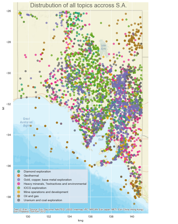
And there you have it, the spatial distribution of each of our located exploration reports, colour coded by topic. But this presentation is not all that useful to see spatial trends in the data. We could plot each topic individually, but a better representation I think is to grid the data.
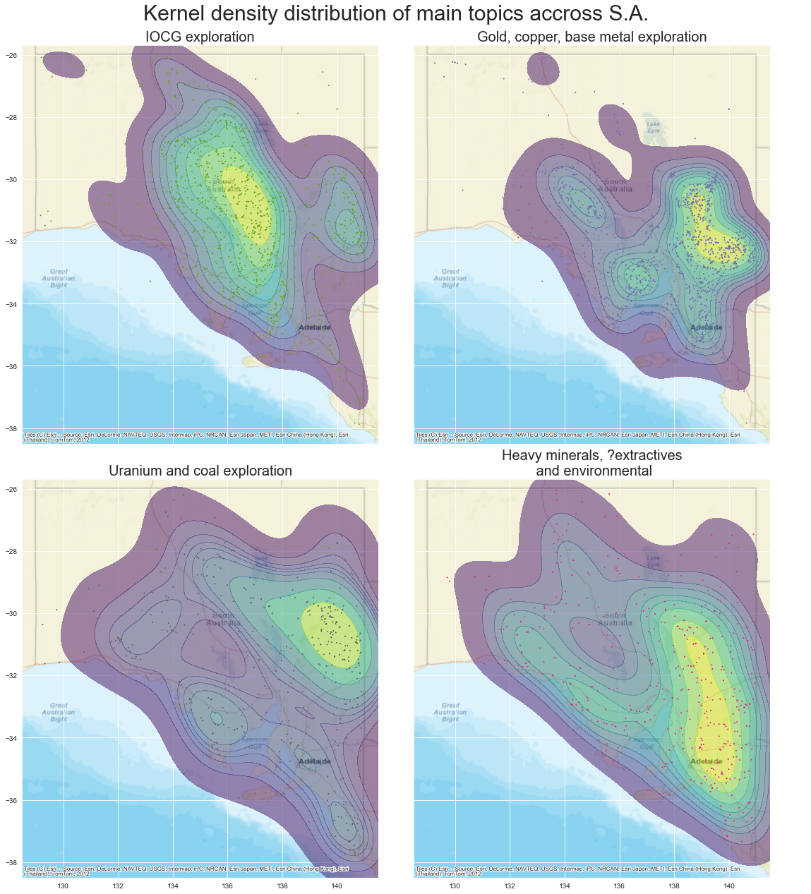
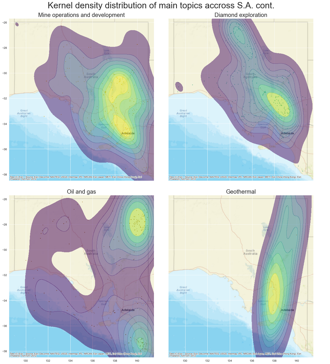
This is where the geoplot library comes in. Geoplot is a high level geospatial data visualisation library that makes plotting data on maps easy. There are a number of differnt plot types avaliable in geoplot but we’re after their kernel density estimation (KDE) plot, kdeplot.
A kernel density estimation is is a useful way to observe the shape of a distribution of data. It is a non-parametric estimation of the probability density function of our topic points. For our one-dimensional data, essentially each data point is assumed to be a normal gaussian distribution centred around that point, then those distributions are summed to create the KDE curve. In the below figures, the more yellow represents areas with a high probability of data points, while the blue is low probability. You’ll see I also included the point data on each of the plots for reference as well.
For ease of viewing, I created two seperate images each containing four maps. The code below to create these images is only for one of the figures, but the full code is avaliable from the GitHub repository.
uranium = all_tenement_topics_nodup_gdf.query("Dominant_Topic == 0")
iocg = all_tenement_topics_nodup_gdf.query("Dominant_Topic == 1")
base = all_tenement_topics_nodup_gdf.query("Dominant_Topic == 2")
diamond = all_tenement_topics_nodup_gdf.query("Dominant_Topic == 7")

fig3, ax3 = plt.subplots(2,2, figsize=(18.4,20.1), sharex=True, sharey=True, gridspec_kw={'wspace':0.1, 'hspace':0.09})

for r in range(2):
    for c in range(2):
        ax3[r,c].set_xlim(128.5,141.5)
        ax3[r,c].set_ylim(-38.456,-25.6)
gplt.kdeplot(iocg, ax=ax3[0,0], cmap='viridis', shade=True, alpha=0.5)
gplt.pointplot(iocg, ax=ax3[0,0], s=1, color= '#66A61E')
ax3[0,0].set_title("IOCG exploration", fontsize=20)
gplt.kdeplot(base, ax=ax3[0,1], cmap='viridis', shade=True, alpha=0.5)
gplt.pointplot(base, ax=ax3[0,1],s=1, color='#7570B3' )
ax3[0,1].set_title('Gold, copper, base metal exploration', fontsize=20)
gplt.kdeplot(uranium, ax=ax3[1,0], cmap='viridis', shade=True, alpha=0.5)
gplt.pointplot(uranium, ax=ax3[1,0],s=1, color='#666666')
ax3[1,0].set_title('Uranium and coal exploration', fontsize=20)
gplt.kdeplot(hm, ax=ax3[1,1], cmap='viridis', shade=True, alpha=0.5)
gplt.pointplot(hm, extent=extent, ax=ax3[1,1],s=1, color='#E7298A')
ax3[1,1].set_title('Heavy minerals, ?extractives\n and environmental', fontsize=20)
for r in range(2):
    for c in range(2):
        ctx.add_basemap(ax3[r,c], crs=all_tenement_topics_nodup_gdf.crs.to_string(), source=ctx.providers.Esri.WorldStreetMap, aspect='auto')
        ax3[r,c].axison=True
fig3.subplots_adjust(top=0.94, left=0.1)
fig3.suptitle("Kernel density distribution of main topics accross S.A.", fontsize=30)
plt.tight_layout()
plt.show()
What does it all mean
So what can we make of the above KDE spatial distribution plots of our modelled topics. To me this is a great way to see how different parts of the state have been the focus for different commodities. Knowing about the geology of South Australia, this also validates the modelled topics and the usefulness of this technique.
For example, we can see that ‘IOCG exploration’ is centred and focused around the eastern Gawler Craton region where we would expect it to be, with some IOCG exploration also focused in the Curnamona Province in the states east. ‘Gold, copper and base metal exploration’ on the other hand is more focused in the northern Flinders Ranges and Curnamona regions, where there has been significant modern and historic mineralisation and exploration potential, with deposits like the Burra copper mine and the base metal exploration in the Curnamona looking for another Broken Hill Pb-Zn deposit. It also highlights the gold, copper-gold and silver focused exploration around the Tarcoola region and the upper Eyre Peninsula. Similarly uranium exploration is focussed on the Mount Painter/Lake Frome region which hosts the Beverly U deposit and Oil and Gas are focused largely around the Cooper and Otway Basins in the states north-east and south-east respectively.
An interesting outcome for me is the distribution of both the ‘mine operations and development’ and the ‘heavy minerals, ?extractives and environmental’ topics. When I generally think about mining in South Australia, I’m drawn to the recent mining opperations associated with the IOCG deposits like Olympic Dam, Prominant Hill and Carrapateena. But the distribution of mine related topics is strongly focused around the northern Adelaide, upper Yorke Peninsula and Flinders Ranges regions. I think this reflects the ongoing exploration and discussion around the mining history and still real exploration potential of the copper triangle and historic mining regions of Moonta, Wallaroo, Kapunda and Burra. Simarly for the heavy-minerals and extractives topic. Modern heavy minerals exploration is focused in the south-west of the state, which is highlighted by the topic distribution, but the dominant region is around the Mount Lofty Ranges, Adelaide and the lower Flinders Ranges. I think this reflects the extent of the extractives exploration around the built up and populated parts of the state (extractives are things like dimension stone for building, limestone for concrete and quarries for road base and construction material etc) and gives me more confidence that the model is indeed picking up extractives as a strong part of that topic (and that I should take that ? out of the topic name!).
Summary
My aim and hope is that this, and the previous article on topic modelling, has given you some insight into the potential hidden information that is contained in the large textural datasets held by the GSSA, and how we might use python and its ecosystem of data science and visualisation tools to easily access those insights. By applying the unsupervised LDA topic model to the exploration report abstracts, it becomes clear that the bulk of the exploration activity that has occurred in South Australia can be classified into one of eight different themes. Then by using some simple python data science and visualisation tools like geopandas, geoplot and contextily we can quickly create spatial visualisations of this data to get a real sense of not just what are explorers looking for in South Australia, but where are the looking.
I hope you’ve enjoyed reading this. Please check out my other content at GeoDataAnalytics.net, and get in touch if you have any questions or comments. And make sure you check out all the amazing freely avaliable data from the Geological Survey of South Australia, SARIG and the SARIG data catalog. All the code used to undertake this analysis is available from GitHub.