
What are explorers looking for in S.A.? Part 1

Finding topics in exploration reports using natural language processing.
When people think about data, often they think about tabular data sets of numbers. But there is a wealth of data and knowledge hiding in unstructured textural data sets such as company exploration reports. Natural Language Processing (NLP) is the field of machine learning concerned with, amongst other things, extracting data and insight from documents. One of the major subdomains of NLP is trying to automatically extract the topics or themes discussed in large volumes of text. Topic modelling is a form of unsupervised learning that tries to identify hidden themes in textural data. As such, there is no need to have labeled datasets to train a model on, it can be applied directly to a set of documents to automatically extract information.
In this first of a two part blog, I will explore one application of NLP topic modelling using Latent Dirichlet Allocation and the gensim library to see if we can identify the main exploration themes in South Australian company exploration report summaries. In the following post, I will explore how to spatially asses the distribution of these topics using the geopandas and geoplot python libraries.
All the code used to create and preprocess the data set, undertake the topic modelling and spatially analyse the results can be found here: SA-exploration-topic-modelling.
What is Latent Dirichlet Allocation?
Latent Dirichlet Allocation (LDA) is a generative probabilistic model that represents a document by identifying latent (hidden) topics (Blei et al., 2003). The basic premise is that each document in a corpus (collection of documents or texts) can be represented by a distribution of topics, where each topic can be represented by a distribution of words.
The LDA model is based on an Bayesian inference framework. The model assumes that each document is composed of a certain proportion (distribution) of a fixed $K$ number of topics, which in turn is made up of a certain proportion of words in that document. To find the hidden topics the LDA model needs to learn the topic representation of each document and the words associated with each topic. It does this by first randomly assigning each word in the documents to one of the $K$ topics. This gives an initial representation of both the topic distribution of the documents and the word distributions of all the topics. The algorithm then iterates through all words in each document and updates the probability that that word belongs to that topic based on: $$p(topic_t | document_d) * p(word_w | topic_t)$$ where:
$p(topic_t | document_d)$= the proportion of words in document$d$currently assigned to topic$t$, and$p(word_w | topic_t)$= the proportion of word$w$assignments to topic$t$over all documents
After iterating across all words in all documents a large number of times, the model will eventually converge on the most likely topic and word distributions.
It’s important to note that the number of topics $K$ is not derived but needs to be provided as a prior. Also the derived word distributions for each topic will need to be labeled as a coherent human understandable topic. I will discuss each of these aspects below.
The data
It is a requirement of legislation that exploration companies operating in South Australia submit reports and data on their exploration activities. These reports come in the form of technical documents and can contain multiple modalities of data including maps, geochemical data and written exploration reports. The South Australian Government has ~ 8000 of these digital exploration ‘envelopes’ or reports on mineral and petroleum exploration and activities dating back to the 1950’s. These envelopes can range in size from a few pages to over 10,000 pages in length.
These data are all publically available via the SARIG web portal. In addition to the full pdf and OCR’d text versions of the envelopes, the Geological Survey of South Australia (GSSA) has indexed these reports and provides a csv tabular data set which includes the envelope number (the document ID), the tenement number associated with the report, a broad subject and a short summary or abstract of the report, along with a number of other metadata columns. The important data column for this work was the abstract column, consisting of a short text summary of the envelope created by a GSSA geologist. Below is a random example of one of these abstracts from ENV09474:
An area covering parts of west-central Lake Torrens and Andamooka Island was taken up by Pima Mining because it was considered a strategic acreage acquisition, since it adjoins the southern boundary of the company's EL 2528 Andamooka already issued to cover a more northerly part of Lake Torrens. Subsequently commissioned aeromagnetic and other geophysical data interpretations made by specialist consultants identified a significant, 18 km x 12 km magnetic anomaly occupying the northern end of the subject tenement, EL 2533, and extending into EL 2528. It coincides with a 17 mGal amplitude Bouguer gravity anomaly - for comparison, the Olympic Dam orebody is associated with a 12 mGal gravity anomaly. This primary target is coincident with the Torrens Hinge Zone, and abuts the Olympic Dam Tectonic Corridor to the north-west. It is believed to have the potential to host a large-scale, economic Cu-U-Au deposit comparable to Olympic Dam. Initial reconnaissance surface rock chip geochemical sampling (6 samples) carried out in the south-western portion of the licence area failed to identify any significant gold or base metal anomalism. However, re-assaying of drill core from historic diamond hole TD2 drilled in late 1981 by Western Mining Corp. returned significantly anomalous copper values including 9.5 m @ 0.4% Cu, 3 m @ 1.15% Cu and 7.5 m @ 0.23% Cu. Other anomalous trace metal values that were detected included 0.5 m @ 77 ppm Ag and 1 m @ 0.25% Pb. Processing of high resolution aeromagnetic profile data covering the Bosworth licence area was performed with the aim of generating a three-dimensional picture of the magnetic basement and defining the positions of major crustal lineaments. Four main structural features were identified that appeared to persist with depth, one striking north-northwest, the second striking north-west, the third north-east and the fourth west-northwest.
Of the ~ 8000 digital exploration envelopes, there are 5894 abstracts provided in the dataset which I’ve used in the topic modelling analysis.
Preprocessing and exploratory data analysis
Before applying any NLP technique to a document, there are a number of text preprocessing steps required to clean up the data set and make it suitable for modelling. For this data set I applied the following text preprocessing steps:
- First convert the character encoding to utf-8 to remove any potential accented or non-ascii characters and then lowercase all characters.
- Remove any extra new-lines, white-spaces or tabs.
- Lemmatise the words using the
spacyNLP library. Lemmatisation is the process of converting a word to its base form, for example the lemma of ‘running’ and ‘ran’ is the word ‘run’. - Remove any special characters, punctuation, digits and single characters.
- Remove stop words using the NLTK library. Stop words are common words like ‘me’, ‘we’, ‘them’, ‘the’, etc, which are common but add no real information to the text analysis.
- And finally convert all words to tokens, i.e. a list of individual words.
After preprocessing, our above example abstract now looks like this:
['area', 'cover', 'part', 'west', 'central', 'lake', 'torrens', 'andamooka', 'island', 'take', 'pima', 'mining', 'consider', 'strategic', 'acreage', 'acquisition', 'since', 'adjoin', 'southern', 'boundary', 'company', 'el', 'andamooka', 'already', 'issue', 'cover', 'northerly', 'part', 'lake', 'torrens', 'subsequently', 'commission', 'aeromagnetic', 'geophysical', 'data', 'interpretation', 'make', 'specialist', 'consultant', 'identify', 'significant', 'km', 'km', 'magnetic', 'anomaly', 'occupy', 'northern', 'end', 'subject', 'tenement', 'el', 'extend', 'el', 'coincide', 'mgal', 'amplitude', 'bouguer', 'gravity', 'anomaly', ...]
Now we can do some simple exploratory data analysis (EDA) using the pandas python library to have a look at the data we have to play with. Looking at some of the metadata provided we can see that the reports have already been classified into nine unique but slightly overlapping categories:
print(df['Category'].unique())
['Company petroleum exploration licence reports' 'DSD publications'
 'Non-DSD publications, theses and miscellaneous reports'
 'Company mineral exploration licence reports' 'Departmental publications'
 'External publications, theses and miscellaneous reports'
 'Company mining program' 'Mineral Production Licence report'
 'Geothermal exploration licence reports']
Of the 5892 abstracts in the database, only 5465 of them have an associated tenement number. This will affect our spatial analysis later on because it means we can’t link every report to a physical location.
Looking at our abstracts we can see that they range in length between a measly single word, up to a respectably detailed 2437 words long. Because LDA topic modelling is based on the frequency of words in the texts, it might be interesting to see what the most common words are, and how many we have to play with.
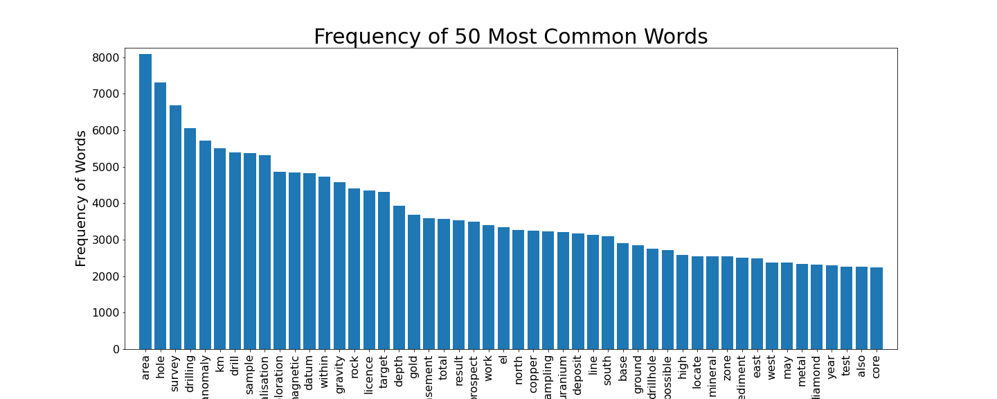
There are a total of 841,074 words in the normalised data set. From the figure above it can be seen that the top 50 words each appear more than 2000 times each. Some of these words, like ‘area’, ‘hole’ or ‘km’ don’t look likely to provide significant, interpretable topics and we could potentially remove some from the data set. But I decided to try to model the entire dataset as is, with the option to further ‘clean’ the dataset if the modelling was not clear.
Creating the LDA model
The first step in creating the LDA model is to identify phrases in the data set. Bigrams and trigrams are phrases made up of two and three words respectively that frequently occur together and make more sense as a single phrase than separate words. Examples from this data set include phrases like murray_basin, natural_gas and anticlinal_structure which, when included as a combined ‘token’ instead of single words, conveys semantic meaning.
The gensim library provides a Phrases model which can generate n-grams by calculating statistics for how often two (or three) words occur together (collocation) in the given corpus. Any given collocation of words will be concatenated as an n-gram based on if a scoring parameter (in this case the default function based on Mikolov et al., 2013) is above a set threshold. First we train the bigram and trigram models on the corpus and then generate the new dataset that includes them:
data_words = df.Abstract_toks.to_list()

bigram = models.Phrases(data_words, min_count=5, threshold=30)
trigram = models.Phrases(bigram[data_words], threshold=100)
bigram_mod = models.phrases.Phraser(bigram)
trigram_mod = models.phrases.Phraser(trigram)

def make_trigrams(texts):
    return [trigram_mod[bigram_mod[doc]] for doc in texts]

data_words_trigrams = make_trigrams(data_words)
The next step is to create the word embeddings to feed into the LDA model. Word embeddings are the vector representation for each word in a corpus (i.e. a numerical representation of a word that the model can use). Because the LDA algorithm only uses word frequencies, and doesn’t take the position of a word in a sentence or the surrounding words into account, it uses a bag-of-words (BoW) model to generate vectors for each document.
First we compute a dictionary mapping assigning an integer ID to each unique word in the corpus. This dictionary will allow us to map back to the original words as well as indicate the total number of unique words in the corpus. We can then convert each document to a BoW, which will represent each document as an n-dimensional sparse vector, where n is the total number of unique words in the corpus. Each element of the vector is a tuple of the word id and the word count in the document:
# Create Dictionary
id2word = corpora.Dictionary(data_words_trigrams)

# Term Document Frequency
corpus = [id2word.doc2bow(text) for text in data_words_trigrams]
Finally we can train our LDA model by implementing the gensim LdaModel class:
Lda = models.LdaModel
lda_final = Lda(corpus, num_topics=8, id2word=id2word, passes=20, chunksize=2000,random_state=43)
Determining the optimal number of topics
As mentioned earlier, one of the priors that needs to be provided to the LDA model is the number of topics, $K$. There are a number of ways to evaluate the derived topic models. We can try to optimise the number of topics by using a measure such as perplexity or coherence (which is a measure that uses the conditional likelihood of the co-occurence of words in a topic and therefore captures some of the context between words in a topic, producing more human understandable outputs).
To optimise the number of topics we need to train an ensemble of LDA models with a range of values for $K$ and calculate the coherence measure of each. In this case I have used the ${C_v}$ coherence measure of Roder et al. (2015):
Lda = models.LdaModel
coherenceList_cv = []
num_topics_list = np.arange(3,12)
for num_topics in tqdm(num_topics_list):
    lda= Lda(corpus, num_topics=num_topics,id2word = id2word,
            passes=20,chunksize=2000,random_state=43)
    cm_cv = CoherenceModel(model=lda,
                            texts=data_words_trigrams, dictionary=id2word, coherence='c_v')
    coherenceList_cv.append(cm_cv.get_coherence())
Plotting these results we can see that our coherence measure increases until about 8 topics, where it then plateaus before ramping up again.
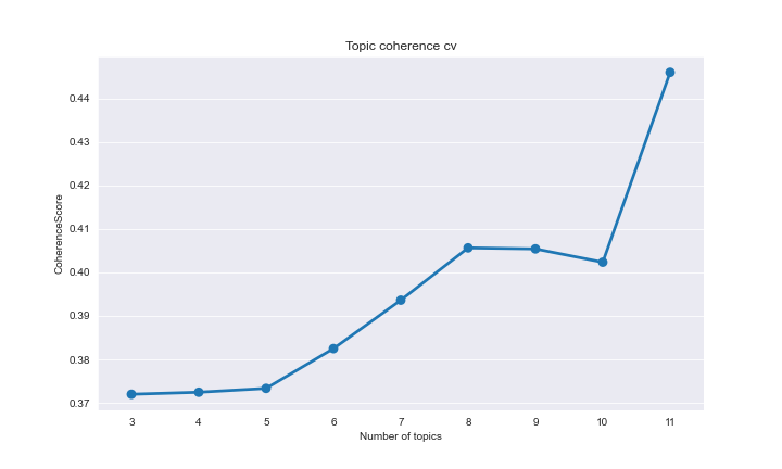
The idea here is to find the ideal number of topics by maximising the coherence value. In this case even though 8 topics is not the maximum value, the fact that it plateaus for nine and 10 topics before increasing again at 11 topics suggests eight is the ‘lowest’ optimal number. Adding more topics can be useful to find norrower topics or even sub-topics within themes, but can also add noise.
The best way to then asses the true ‘clarity’ or understandability of the various topics produced by the models is through visualising them and assessing the most relevant terms in each topic. If there is too much overlap between the topics that may suggest we have modelled too many. A great tool to visualise the produced topic space is the pyLDAvis python library.
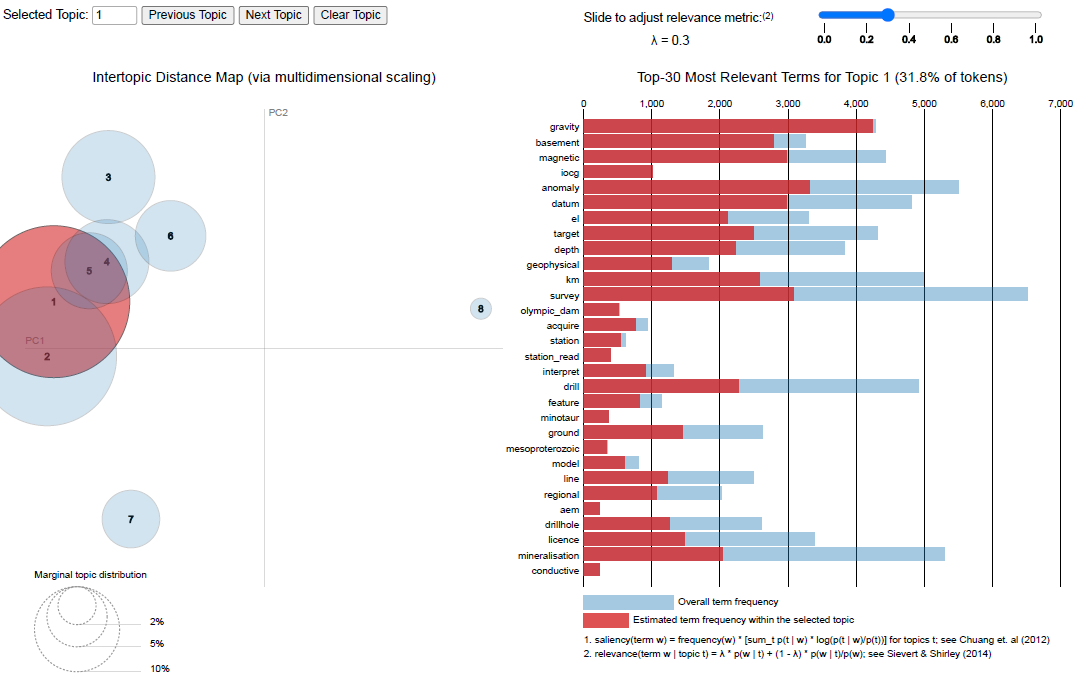
You can play with an interactive version of this visualisation here. This visualisation tool allows us to asses how similar the topics are in vector space, see the top 30 highest likelihood words, and also adjust the variable $\lambda$ to asses the most relevant words in a topic.
After assessing the coherence measures and visually reviewing the derived topic word lists, I settled on eight as the optimal number of topics to describe our exploration envelope abstracts.
What are the modelled topics
The output of the LDA models are essentially a list of words, from the corpus, that are ascribed to each of our eight topics. It still requires an assessment of just what those topics are actually describing. This is where a bit of domain knowledge comes in.
From the model we are able to extract both the most probable words in each topic, the relative frequency of each topic across the corpus and importantly, we can also extract the most relevant words to each topic (Sievert & Shirley, 2014). By adjusting the value of $\lambda$ in the relevancy function, we can get a much clearer idea of what the topic is actually describing. This works by essentially showing the less-common words that are only relevant to a specific topic.
When we set the $\lambda$ value to something like 0.3 we get the following relevant words for each topic:
| Topic | Relevant words | Frequency |
|---|---|---|
| Topic_0 | [uranium, coal, sand, tertiary, clay, lignite, channel, palaeochannel, sedimentary_uranium, groundwater, eyre_formation, rotary, beverley, gamma_ray_log, talc, seam, radioactivity, sediment, radio.. | 9.700699 |
| Topic_1 | [gravity, basement, magnetic, iocg, anomaly, datum, el, target, depth, geophysical, km, survey, olympic_dam, acquire, station, station_read, interpret, drill, feature, minotaur] | 31.822340 |
| Topic_2 | [gold, soil, sample, rock_chip, copper, value, sampling, au, base_metal, mineralisation, anomalous, geochemical, return, assay, vein, prospect, ppm, zone, bedrock, calcrete] | 26.565557 |
| Topic_3 | [gel, geothermal, gel_grant, desktop, heat, surrender_th, thermal_conductivity, energy_ltd, vacuum, hot_dry, nd, commit, hot, heat_produce_granite, impasse, munyarai, ddcop, nicul, mount_james, sa… | 0.610204 |
| Topic_4 | [resource, mining, iron_ore, ore, sub_block, recovery, grade, plant, hillside, technical, metallurgical, mine, iron, resource_estimate, year, beneficiation, cost, concentrate, orebody, havilah] | 11.915023 |
| Topic_5 | [seismic, pel, petroleum, kms, survey, gas, hydrocarbon, reservoir, epp, oil, closure, moomba, comprise_detail_operation_field, cooper_basin, record, line, otway_basin, velocity, mature, acquisiti… | 6.855799 |
| Topic_6 | [hm, relinquish, iluka, licence, heavy_mineral, gypsum, relinquish_portion, surrender, strandline, magnesite, portion, murray_basin, eucla_basin, iluka_resource, dune, ooldea, tenement, hms, beach… | 7.949810 |
| Topic_7 | [kimberlite, foot, mineralization, indicator_mineral, kimberlitic, aerial, diamond, loam, kimberlite_indicator_mineral, grain, fdl, cattlegrid, microdiamond, kimberlitic_indicator_mineral, stockda… | 4.580569 |
From the above lists of relevant words it becomes apparent that the eight topics that model the South Australian exploration report abstracts, and therefore the broad themes of exploration in the state over the past 50 years can be labeled as something like:
- Uranium and coal exploration
- IOCG exploration
- Gold, copper and base metal exploration
- Geothermal exploration
- Mine operations and development
- Oil and gas
- Heavy minerals and extractives mining and exploration, and
- Diamond exploration
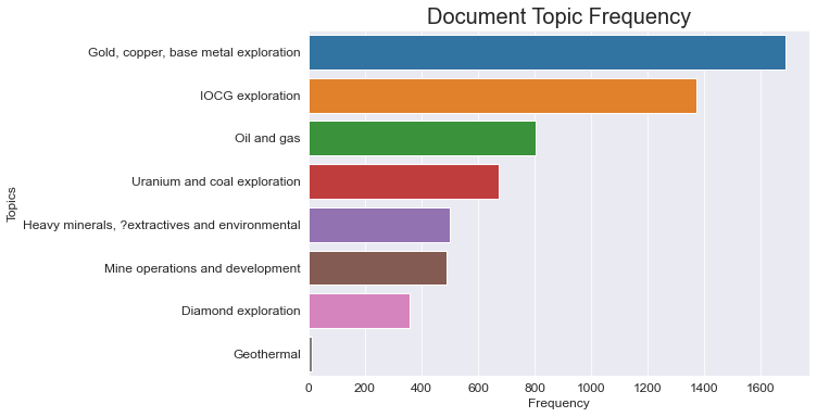
In the table above we show a value for the relative frequency for each derrived topic, i.e. the percentage of documents in the corpus that can be described as having that topic as the dominant theme. We can represent that as an absolute by plotting the number of documents that have each topic as the dominant topic. The plot below clearly shows that the corpus is dominated by the ‘gold, copper and base metal exploration’ and ‘IOCG exploration’ themes, with ‘geothermal’ only making up a small percentage of the exploration in SA.
By looking at the similarity of some of these topics, it is easy to see that there is potentially some broad overlap between things like ‘IOCG exploration’ and ‘gold, copper and base metal exploration’ and between the ‘uranium and coal’ and ‘heavy minerals and extractives’ topics (refer to the pyLDAvis figure above showing the overlap between these topics in vector space). This is to be expected given the significant similarity in the types of methods and reporting undertaken in each type of exploration program. It is also the case that each document may contain more than just the one dominant topic shown above. It’s important to remember that LDA modelling assumes a document is made up of a distribution of topics, not neccisarily a single topic.
By plotting the distribution of the percentage value for each dominant topic for each document in the corpus (i.e. the ‘percentage’ of each document that that topic represents) we can get a picture of how much overlap exists in the data set.
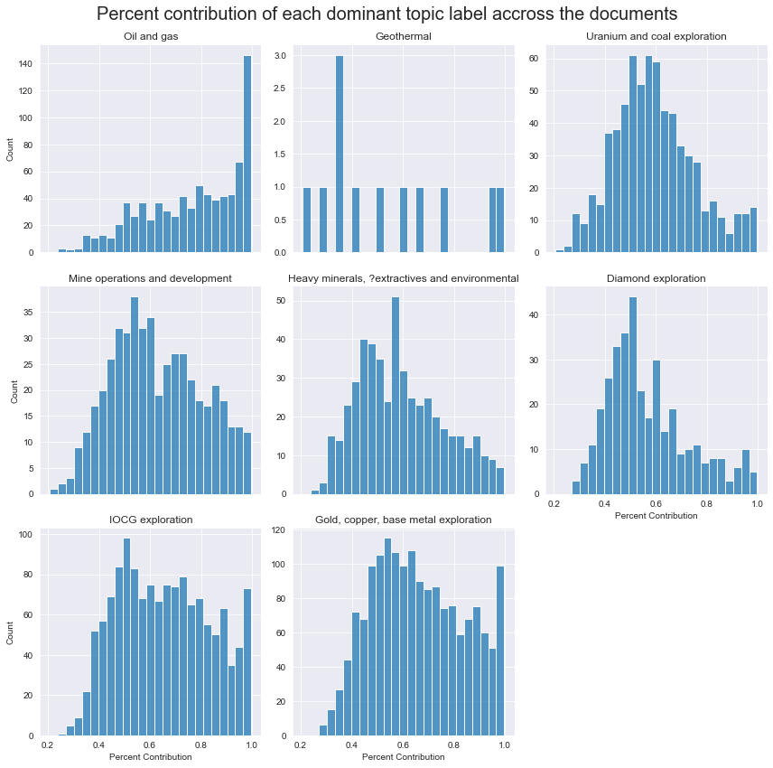
Most of the topics display a positive skewed normal distribution peaking at around 50%. This shows that very few documents are dominated by only one topic, and most are likely mixtures of derrivedmilar topics. The exception to this is the ‘oil and gas’ topic which has more of an exponential distribution with a high percentage of 100% ‘oil and gas’ topic only documents.
Comparison with document classes
FInally we can compare the dominant topics derived from the LDA model with the provided document classifications. As mentioned earlier, one of the meta data coluns in the data set includes a document category. While these categories are not the same thing as the modelled topics, they can provide some insight into how well the model is working for some topics that are close to one of the categories, or what the different publication categories tend to be focused on.
The data set contains nine overlapping categories (see above). The first thing to do is to map these to distinct categories. I have pulled out six distinct categories which include:
- Petroleum exploration publications
- Departmental publications
- Theses and non-departmental miscellaneous reports
- Mineral exploration publications
- Mining related publications, and
- Geothermal publications
We can then make an assesment of how many reports there are that fall into each of these new normalised categories.
final_LDA_df['normalised_category'].value_counts()
    Mineral exploration publications 4597
    Petroleum exploration publications 911
    Departmental publications 167
    Theses and non-departmental miscellaneous reports 137
    Geothermal publications 76
    Mining publications 6
We can see that Mineral Exploration publications dominate, followed by petroleum publications and then a small number of documents from the other classes. Next we can plot the number of documents represented by each dominant topic by each documant category.
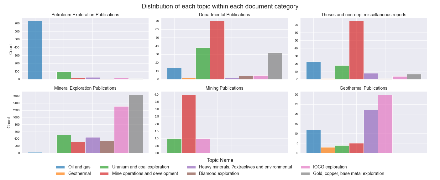
There are a few things we can pull out of this plot. Firstly, for the three categories that can be related directly to one of the derrived topics, ‘oil and gas’, ‘geothermal’ and ‘mine operations and development’. We can see that the model has done a good job in recognising the dominant theme in both the Petroleum exploration publications and the Mining publications. The large intertopic distance between the ‘oil and gas’ topic and the other topics (refer the pyLDAvis figure above), and the positive ‘exponential’ spread in the dominant topic distribution suggests there is significant difference between the methods, the way the reports are written and the terminology used by the petroleum industry compared to the rest of the mining and exploration industry.
For those documents classed as Geothermal publications though, there are mixed results. The model only classified 12 abstracts as being dominated by the ‘geothermal’ theme, with more than half of them having a dominant topic percentage of less than 50%. The LDA model has poentially missclassified a number of geothermal related publications into mostly the ‘IOCG exploration’, ‘heavy minerals, extractives and environmental’ and the ‘oil and gas’ topics. This is despite the apparently large intertopic distance between the ‘geothermal’ topic and the other toipcs. One potential explanation for this may be the relatively juvenile nature of the geothermal exploration industry and the potential mixing between teminology and methodology used in the oil and gas industry and the mineral exploration industry, making some of the geothermal related publications more similar to other topics, at least to the point that the geothermal topic was no longer the modelled dominant topic.
Finally the figure provides some insight into the types of reports and publications produced by the Department and by universities and other consultants. Departmental publications are dominated by ‘mine operations and development’ reports, followed by ‘uranium and coal’ and ‘gold, copper and base metal’ topics. University theses and other reports are also largely focused on the ‘mine development and operations’ topic, probably associated with deposit studies, as well as ‘oil and gas’ which is likely due to the Australian school of petroleum being based in Adelaide and working closely with local oil and gas explorers.
Summary
While the results of this topic model analysis may not be entirely unexpected given a knowledge of South Australian exploration and mineral potential, this article was designed as an example of the potential hidden information that is contained in the large textural datasets held by the GSSA. By applying the unsupervised LDA topic model to the exploration report abstracts, it becomes clear that the bulk of the exploration activity that has occurred in South Australia can be classified into one of eight different themes. This approach could also be applied to different text datasets, such as GSSA report books, or internal company reports to asses what the hidden themes are in those data.
In the next part of this two part blog, I will show how we can use the exploration tenement data associated with each exploration envelope to obtain a spatial location linked to each report. We can then use python to spatially visualise and asses the distribution of the modelled topics, to see what regions each topic applies to.
I hope you’ve enjoyed reading this. Please check out my other content at GeoDataAnalytics.net, and get in touch if you have any questions or comments. And make sure you check out all the amazing work and freely data available from the Geological Survey of South Australia and SARIG. All the code used to undertake this analysis is available from GitHub.